Get Started

library(dplyr, warn.conflicts = FALSE)
library(ggplot2)
library(sf)
#> Linking to GEOS 3.10.2, GDAL 3.4.1, PROJ 8.2.1; sf_use_s2() is TRUE
library(ggspatial)
theme_set(theme_minimal())
library(asds2024.nils.practical)

This package contains a practical project for a university course on data analytics. There’s some data, analyses that were performed on that data, and some miscellaneous utilities and info snippets.

To get a first overview of the data, have a look at its documentation, e.g.

?tracks

or maybe plot it:

be_fr <- swiss_cantons |>
  filter(KTNR %in% c(2,10)) # 2 = BE, 10 = FR
be_fr_lakes <- swiss_lakes |>
  filter(grepl("Biel|Brienz|Gruyère|Murten|Neuchâtel|Thun", GMDNAME)) # only show lakes named after these towns

track_details |>
  filter(!is.na(latitude) & !is.na(longitude)) |>
  st_as_sf(coords = c("longitude", "latitude"), crs = "WGS84") |> # EPSG 4326 = WGS-84
  st_transform(crs = 2056) |> # EPSG 2056 = CH-1903+/LV95
  to_linestrings() |>
  ggplot() +
  geom_sf(data = be_fr, fill = "#f0f0f0", alpha = 0.5) +
  geom_sf(data = be_fr_lakes, fill = "#0080ff", alpha = 0.25) +
  geom_sf(color = "red", linewidth = 0.25, alpha = 0.2) +
  annotation_scale(
    location = "br",
    height = unit(0.1, "cm"),
    width_hint = 0.2) +
  annotation_north_arrow(
    location = "tr",
    width = unit(1, "cm"),
    height = unit(1, "cm"),
    pad_x = unit(0.5, "cm"),
    pad_y = unit(0.5, "cm"),
    style = north_arrow_fancy_orienteering,
    which_north = "true")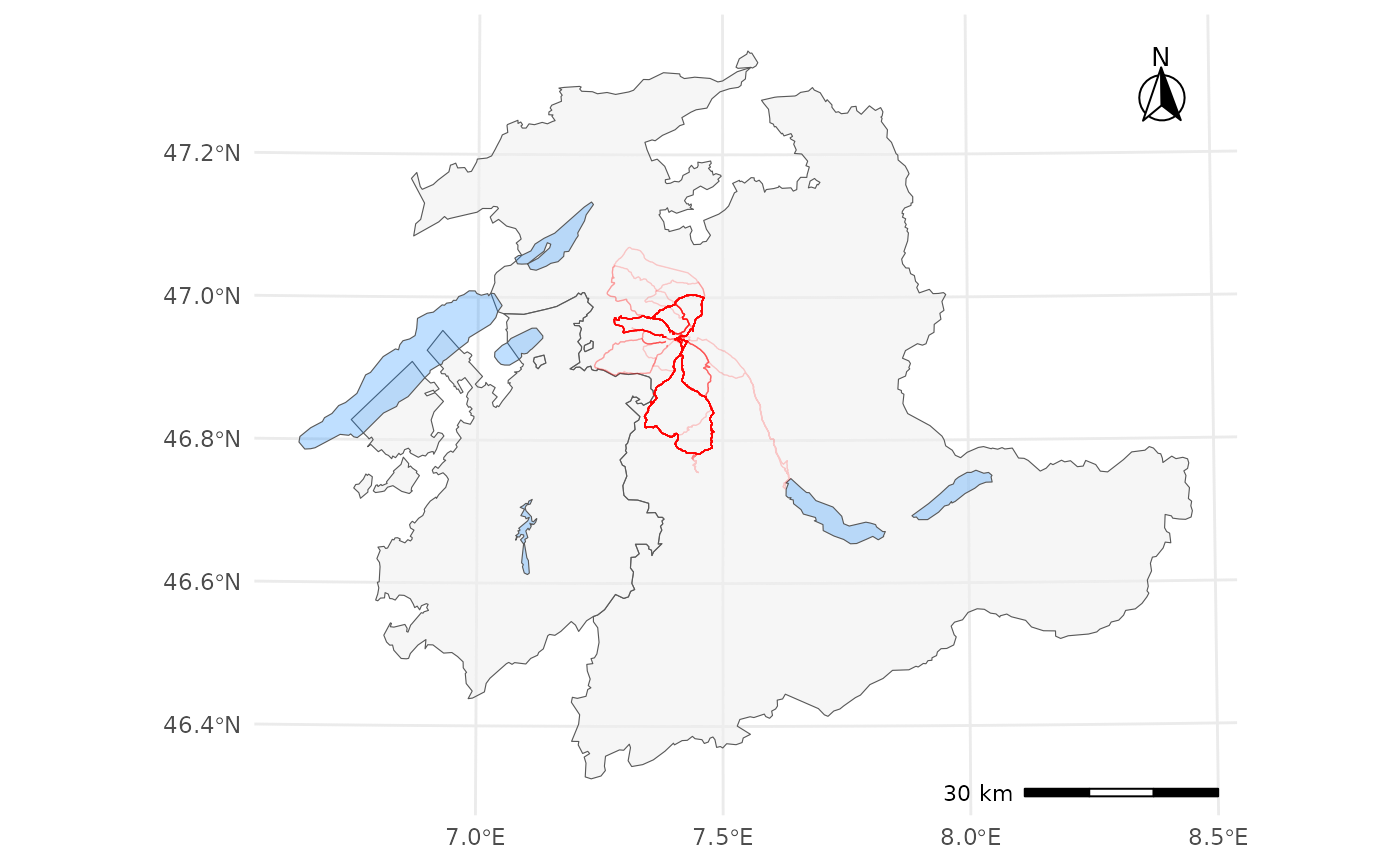

To learn more about the data, see vignette("data").

To see the analyses that were done on the data, see vignette("analyses").

And to get a brief summary of the purpose of this package, see vignette("about").