Exploratory Analysis of Road Bike Trip Data

CAS Advanced Statistical Data Science 2024

Nils S.

30.08.2024

Abstract

For the final project of the CAS program Advanced Statistical Data Science, a real world data set of our own choosing was to be analyzed, using methods learned in class.

This report represents an exploratory analysis of road bike data collected during the bike seasons from 2018 to 2023, using different statistical means to try to find statistically-significant patterns or anomalies in the data.

Introduction

The final module of the CAS ASDS is a practical project. The topic of the project can be freely chosen by the students, e.g. using data from their work environment or from elsewhere.

The data I chose for my final project is data collected from road bike trips during the years 2018 to 2023. Data was collected using a GPS-enabled bike computer, with complementary sensors for heart rate, cadence, and speed data. In total, the preprocessed data comprises approximately 160000 data points, collected during 157 trips. The actual number of trips during those seasons was higher, however, due to a data corruption in the bike computer’s memory, an unknown number of trip recordings was lost. Figure shows the number of tracks for each year in the data set, suggesting that a data block (or data blocks) containing records for 2022 and 2023 was lost.

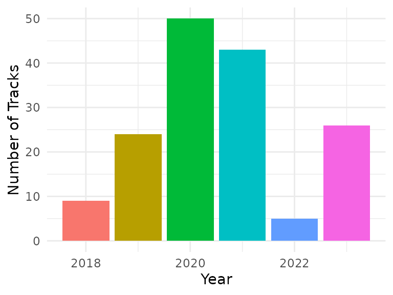
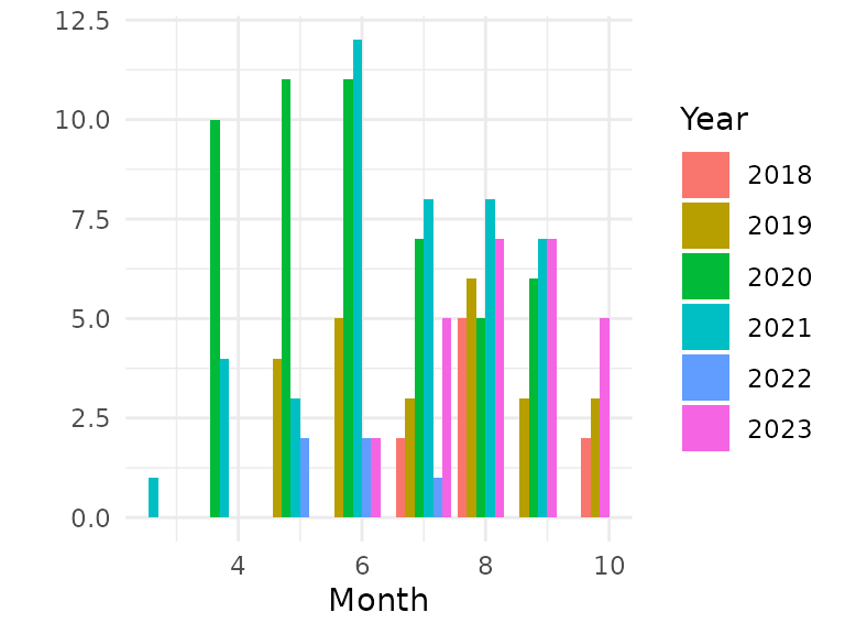
Available trip data by year and month

Figure shows the geographic component of the available data on a map, with the tracks in red. Routes driven more frequently appear more saturated, rarely-driven routes appear lighter (e.g. the route to lake Thun only appears once in the data set).

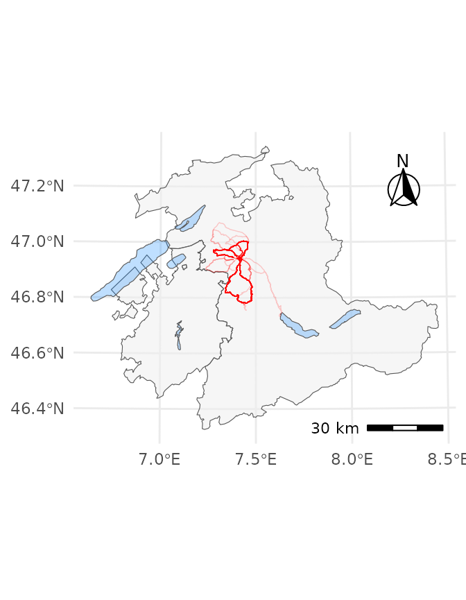
Geographic track data (in red) on a map of cantons Berne and Fribourg

Since the data was not collected for the purpose of this project, i.e. it is not data from a controlled experiment, it is not as well-formed as would be desirable for an ideal analysis. Instead, the project is an exploratory analysis of available data.

Analyses

The data is a time series, however, due to uneven temporal spacing of the data points, missing values, etc., the methods learned in class could not be used in this case. For this reason other methods were attempted, mainly linear models of different sorts, as introduced in the lectures on mixed-effects models (“Lineare gemischte Modelle”, Vock (2023)), and analysis of high-dimensional data (“Analyse hochdimensionaler Daten”, Städler (2024)), and some methods introduced in the lecture on unsupervised learning (“Unüberwachtes Lernen und Dimensionsreduktion”, Dümbgen (2024)). These approaches are problematic (due to the data being correlated to some degree, and because the fundamental nature of the data is a time series, which should be analyzed using methods designed for such data), but to get a first impression the analyses performed should still be okay, and their results should still be valid.

The code and some additional description for the analyses can be found in vignette("analyses") for the package accompanying this document. This report will mainly present the results of the analyses, along with remarks and conclusions.

Global Linear Models

The first approach is to fit global linear models, i.e. models using all the data. The focus was finding effects influencing the average speed for a track. Questions I tried to answer were:

• is there an effect of temperature?
• what are the effects of track length, average inclination, and heart rate?
• does a previous track (i.e. the previous training) have a significant impact / what aspect of a previous track has an impact (previous track length/inclination/heart rate, time since previous training, …)?
• is there a training effect over the course of the season, i.e. does the average speed increase over the course of the year?

Temperature Effects

The first model using only the average temperature as a predictor for the average speed did not show any significant effect. The original idea behind fitting the model was based on the subjective feeling that warmer temperatures lead to lower speed. The temperature coefficient in the fitted model does indicate such a tendency, however, it’s p-value is so large that this might be pure chance. Additionally, the coefficient is so small that even if it was significant, temperature fluctuations within reasonable limits would barely influence the average speed. If such a tiny effect is actually present, much more data would be needed to detect it with any degree of statistical significance, however.

Another aspect to consider is that the assumed “lower temperatures mean higher speed” relationship is too simplistic: there is probably an optimal temperature, below which the average speed decreases again. Such a relationship cannot be modeled by simply fitting a straight line to the data.

An attempt was made to fit splines to the temperature data, but that did not result in viable models, either. Slightly better-fitting models could probably have been achieved using splines, however, due to time constraints these ideas were not pursued further. Instead, I focused on trying to find other patterns in the data, since the results obtained when trying to fit a model for the temperature did not seem too promising.

Effects of Distance, Inclination, and Heart Rate

The second model fitted is based on a track’s total distance, average inclination, and average heart rate. Intuitively, this should be a relatively promising model to explain the average speed. The model can then serve as a baseline reference to compare other models to.

This model explains about 58% of the total variance in the data, and shows that average inclination and average heart rate are highly significant predictors. Somewhat contrary to the initial expectation, though, a track’s total distance has no significant effect, at least not for the usual 5% confidence threshold: the distance effect has a p-Value of just above 5%.

The model seems to fit the data relatively well, with some outliers visible in the diagnostic plots. The more obvious outliers are caused by tracks that were rarely driven (e.g. the route of track 2, driven on July 31st, 2018, was only driven once), highlighting their difference from tracks that were driven frequently.

Effects of Previous Training Sessions

Since one training session can influence a subsequent training session (e.g. because there was not enough time for recovery between sessions, or because after recovering from the first session, the overall fitness was better), an attempt was made to model such an effect. The most important predictors are probably still the track’s distance, inclination, and heart rate, but the previous track’s details (i.e. the previous track’s distance, inclination, and heart rate) were also considered. Additionally, the time between the training sessions was included in the model, so that e.g. for two tracks $t_1$ and $t_2$ driven 2 days apart, the effect $t_1$ has on $t_2$ can be different from the same two tracks being driven 20 days apart.

The fitted model explains about 3% of additional variance in the data when compared to the previous, simpler model. However, only the time since the previous track, and the previous track’s distance are significant. Considering that track distance strongly correlates with the duration of the track, it could seem logical to use the training time of the previous track as a predictor instead of the previous track’s distance, however, that approach produces a model with slightly lower $R^2$, and the previous track’s duration is actually a less significant predictor than the distance.

Overall, though, the extended model is not very useful. It is more complex and less explainable (for example, the average speed decreases with increasing time since the last training, but increases with the previous training’s distance; thus, a track driven the day after driving a very long track should have a higher average speed than a track driven a few days after a shorter track, which does not match past experiences). Additionally, the diagnostics look a bit worse than for the simpler model (the QQ-plot of the residuals looks a bit worse, and the residuals-vs-leverage plot shows some observations with higher leverage than before). All of these drawbacks only result in a model that explains an additional 3% of variance.

Effects of the Training Season

Another approach to take previous trainings into account is to check for effects of the training season: within a given year, have tracks later in the year a higher average speed than tracks earlier in the year? Assuming that the fitness level is lowest directly after the winter, it should rise over the course of the season, i.e. the more training sessions were performed, the higher the fitness level should be. Multiple models were evaluated for this approach, some using the month, and a final one using the calendar week.

Starting with the simplest model of using just the month as a predictor, there is no significant effect. Considering that an increase in fitness probably goes along with driving (on average) longer tracks, which are more exhausting, and therefore reducing average speed, additional predictors are needed to detect the effect of the training progress during the season. Thus, the same predictors used for the basic model were added back, together with their interactions with the month. Thus, for example, depending on training progress during the season (i.e. month), the average heart rate could have a different effect per month. This model already has 32 coefficients, compared to just four coefficients for the basic model. However, three of the coefficients are actually NA values (the interaction effects for October), and of the remaining coefficients, only four (apart from the intercept) are significant (at a 5% confidence level). One of the significant effects is the average inclination (which was already significant in the basic model), the other three significant effects are some of the interaction effects. There is no obvious pattern for which effects are significant (other than the inclination), which makes this model harder to explain than the basic one, while offering the advantage of explaining about 71% of the variance. The diagnostics look a bit worse for the more complex model, though, with the QQ-plot of the residuals slightly worse than for the basic model, and the residuals-vs-leverage-plot noticeably worse.

Attempting to fit a model for the season with higher temporal resolution (using calendar week instead of month) is pointless, though: there is data for 29 different calendar weeks, resulting in 28 coefficients for the calendar weeks alone, plus an additional 28 coefficients for each interaction, and some more coefficients for the other effects, for a total of 116 coefficients. Of those, 15 result in NAs, however, and of the remaining non-NA coefficients, only one is significant. Even the intercept and the inclination are not significant in this model, and the diagnostic plots look clearly worse than those of the basic or month-based models.

The difficulty in finding effects for the training season are probably at least in part caused by lack of data: there are only six seasons for which there is data, and at least for three of those seasons the data is incomplete: for the first year (2018), there is no data for the start of the season (because the bike computer was only bought mid-season), and for 2022 and 2023 there is missing data due to memory corruption in the bike computer, with (at least) the later part of the 2022 season and the beginning of the 2023 season missing. Even if these seasons were completely available, it would still be only six seasons worth of data from which to extrapolate. With the missing data, the choice is between removing the incomplete seasons (and trying to extrapolate from even less data of just the remaining three seasons), or using all data and potentially skewing the results. The latter option was chosen, the former might be something to try in the future. Out of all the training season-based models fitted so far, only the one using the month and its interactions seems usable, however, due to the model’s complexity the basic model still seems like a more robust and useful choice (despite explaining quite a bit less variance).

Lasso Regression using ElasticNet

After fitting the preceding models, which used manually-selected predictors, I tried Lasso regression (Tay, Narasimhan, and Hastie 2023) to see which predictors would be selected. Since there are some more predictors available than those that were used until now, the idea was that if there were important predictors that were not considered, those would now be found by the Lasso regression.

In a first round of Lasso regression, using 12 available predictors to model the average speed, only one predictor (one of the heart rate zones) was eliminated by the Lasso.

This model is still relatively large, and many of the predictors are highly correlated: the heart rate-based predictors are correlated with each other, and a track’s time and distance are also highly correlated. By eliminating correlated predictors (only keeping average heart rate as a heart rate-based predictor, and keeping distance but not time), we reduce the number of available predictors to 5. Trying Lasso regression on the reduced set of predictors results in a model based on distance, inclination, and heart rate. This is exactly the same set of predictors that was already used for the basic model, i.e. the initial selection seems to have been appropriate. This also means, however, that Lasso regression does not really help improve the models created before, it only confirms the gut feeling based on which the basic model was constructed.

Random Effects

A last thing to try for the global linear model is to add random effects (Pinheiro, Bates, and R Core Team 2023). For example, we could assume that a model based on distance, inclination, and heart rate (i.e. the basic model) is a good fit for the data, but that there are slight differences in average speed among the years, e.g. caused by different decreases in fitness during the winter. This could be modelled by a random effect for the year. Another possibility would be a random effect to model differences among different routes that are not explained by differences in route length or inclination. Furthermore, effects could be nested, e.g. there could be a route-specific random effect that varies among years, or there could be additional random effects for the month within each year. The nested effects could explain e.g. a situation where certain routes seem easier in some years, or fluctuations in fitness during the year (i.e. per month).

Fitting such models shows that a model with a random effect for the route is not better than the basic model, however, a model with a random effect for the year is quite certainly better than the basic model. Both nested models (i.e. route in year, and month in year) are also slightly better than the model with just a random effect for the year.

Out of the three mixed models that perform better than the basic model, the simple model with just a random effect for the year is probably the most appealing one: it is the simplest of the three, and a random variation between years seems intuitively plausible. The nested models are only slightly better performance-wise, but harder to understand. Furthermore, the nested random effects appear less intuitive. Considering for example that routes are fixed, a random effect for the route seems less likely than a deterministic, fixed effect for the route. The random effect might just work to compensate for some route parameters that are not available in the data. Similarly, instead of the random effect for the month, some sort of fixed effect would seem more plausible (fitness or training effect of some sort), but again, the random effect might compensate for some relationship that would need additional data to model as a fixed effect.

Principal Component Analysis

After trying to fit linear models to the data with mixed success, I tried to determine the main sources of variance in the data. For this, a principal component analysis was done for 15 variables.

The two most important principal components explain almost 60% of the total variance, with the first component’s main influencing factors being the time, distance, inclination, and altitude gain, and the second component’s main influences being the heart rate-related variables. Considering which predictors were found to be statistically relevant in the linear models, this does not seem surprising.

What was surprising, though, was the biplot of the first two principal components, which showed two clearly separated groups of observations.

Clustering

After seeing the distinct groups of observations in the PCA biplots, the next thing I tried was clustering of the data points.

The first approach was a Gaussian mixture model (Scrucca et al. 2023), which can be fitted without any additional parameters, i.e. given the data it will automatically determine a clustering without any further inputs. The resulting clustering is based on four groups. When looking at the groups in a speed-vs-distance plot, the grouping seems to be based mostly on distance (which, for the given data, is a good indicator for the route).

A second clustering approach that was tried is DBSCAN (Hahsler and Piekenbrock 2023). For this algorithm, a preparatory k-nearest-neighbor distance computation has to be performed, and a value of $\varepsilon$ has to be eyeballed from the resulting plot. Different values for k and $\varepsilon$ were tried, however, most of the time the result was a clustering with only two or three groups (i.e. one or two actual classes, plus one “noise” class). For $k = 1$ and $\varepsilon = 2.1$, three classes and a “noise” class were found. Again, the classes are very clearly based on track distance (even more obviously so than for the Gaussian mixture model).

Considering that the clustering algorithms seem to cluster mostly by track distance, a classification based on a track’s route seems natural. This is the most obvious way of classifying the tracks, especially when considering that some tracks were driven quite often. The route-based classification was therefore added manually, to develop models that can use a track’s route as an additional predictor. Additionally, the route classification was also used for random effects to fit additional mixed-effects models (see section ).

Route-specific Linear Models

With the manually-assigned classes, some of the approaches tried for the global linear models can be retried on a per-class basis. However, since all tracks in a class are trips along the same route, route-specific information like distance or inclination are not useful predictors for these models. Furthermore, there are now substantially fewer tracks which can be used to fit a model. The most frequently-driven route has 55 tracks, with the second- and third-most driven routes having 52, and 10 tracks, respectively. For this reason, only the three most-frequently-driven routes were selected to try to fit a basic model for. A slightly more complex model was only tried for the most frequent route.

The first attempt for a simple linear model used the average heart rate, and temperature to model average track speed, since the other predictors used in the basic global model were not applicable when looking at tracks for the same route. Again, as for the global model, for none of the three routes a significant effect of the temperature can be found. Thus, the only predictor which has a significant effect is the average heart rate, with an increase in average speed of between ca. 0.5 and 1 km/h for every 10 bpm increase in average heart rate. The diagnostics plots don’t look too bad for the routes with > 50 tracks (apart from the residual QQ-plots, which show quite obvious deviations from the diagonal, for one route at the lower end, for the other at the higher end of values). For the route with only 10 observations, however, there is too little data, which becomes obvious in the diagnostics plots. So even though the model for that track shows a significant effect of the average heart rate, the model itself is not useful for making predictions.

Attempting to find a training effect over the course of the season for the most frequent route again finds no significant effect, however, this might at least in part be due to lack of data, considering there is only one month for which there are at least ten observations.

Dynamic Time-Warping

While not by itself a statistical analysis method, dynamic time-warping (Giorgino 2009) can be used to map data points of one track to the data points of another track, making it possible to compare them even when they do not have the exact same number of data points. This could be used to find parts of a route that vary a lot (or very little) among different tracks for that route, and then analyze those deviations. Ideas are to compare all tracks along the same route to a reference track (e.g. the fastest or slowest track), or to compare subsequent tracks to each other. Obvious analysis ideas are, again, looking for influences of temperature or training progress for certain route sections with high variability among tracks, e.g. “does temperature influence performance on particularly steep parts of a route”.

This is still ongoing, however, since the necessary analyses could not be finished in time for the final submission deadline.

Conclusion

While quite a few statistical methods learned during the CAS were applied, the overall outcome of the analysis is not particularly impressive. Conclusions that can be drawn with relative certainty:

• a track’s average inclination, and the average heart rate almost certainly have an influence on the average speed, a track’s distance is less important
• for a given route, tracks with a higher average heart rate tend to have a higher average speed
• temperature seems to have a negligible effect
• from the available data, no improvement in overall fitness over the course of the season can be concluded

The fact that temperature does not seem to have an effect, and that there is no apparent training effect seems surprising (as in: does not correspond to subjective observations), as does the fact that distance seems to have a lower-than-expected influence. However, the strong influence of inclination and average heart rate seems obvious.

What is also clear, however, is that most models do not fit very well, even though more fine-tuning could probably improve most of the models to some degree. This is at least in part because of the (assumed) structure of the data (i.e. most effects probably have some sort of curved shape, with an optimal point from which results taper off in both directions). Another aspect for the suboptimal fit is likely due the fact that the available data is lacking in (at least) two aspects:

• There are simply not enough observations to reliably detect small effects, especially in more complex models; reasons are the data loss for the 2022/2023 seasons, and the fact that data was only collected for six seasons in total
• There are other factors that influence performance, like wind, other exercise sessions, resting periods (sleep etc.), and many more. These factors were not measured, though, so their effects invisibly influence the data in unpredictable ways.

While the lack of data cannot be compensated for, there are still other possibilities to explore. Things to attempt in the future (i.e. after the final submission deadline) are improvements to the linear models (exploring the effect of certain interactions, e.g. distance and inclination, or splines and other curve-shaped fits), continuing to experiment with dynamic time-warping, and taking a look at more advanced time-series models than those that were introduced in the CAS lecture on that topic (Hayoz and Hüsler 2023).

Appendix A - Data

The raw data used for this project was recorded by a GPS-enabled bike computer, paired with a chest strap-style heart rate sensor, and a combined speed and cadence sensor. Data was recorded at five second intervals. The individual tracks (i.e. trip recordings) were exported as CSV files.

The (slightly censored) raw data is available in the sources of the R package accompanying this document. More details about the data can be found in the package’s vignette("data"), or by looking at the documentation for the data directly, i.e. ?tracks, ?track_details, or ?track_classes.

References

Dümbgen, Lutz. 2024. “Vorlesungsskript Unüberwachtes Lernen Und Dimensionsreduktion.” Institut für mathematische Statistik und Versicherungslehre, Universität Bern.

Giorgino, Toni. 2009. “Computing and Visualizing Dynamic Time Warping Alignments in R: The dtw Package.” Journal of Statistical Software 31 (7): 1–24. https://doi.org/10.18637/jss.v031.i07.

Hahsler, Michael, and Matthew Piekenbrock. 2023. Dbscan: Density-Based Spatial Clustering of Applications with Noise (DBSCAN) and Related Algorithms. https://CRAN.R-project.org/package=dbscan.

Hayoz, Stefanie, and Jürg Hüsler. 2023. “Vorlesungsskript Zeitreihenanalyse.” Institut für mathematische Statistik und Versicherungslehre, Universität Bern.

Pinheiro, José, Douglas Bates, and R Core Team. 2023. Nlme: Linear and Nonlinear Mixed Effects Models. https://CRAN.R-project.org/package=nlme.

Scrucca, Luca, Chris Fraley, T. Brendan Murphy, and Adrian E. Raftery. 2023. Model-Based Clustering, Classification, and Density Estimation Using mclust in R. Chapman; Hall/CRC. https://doi.org/10.1201/9781003277965.

Städler, Nicolas. 2024. “Analysis of High-Dimensional Data - Prediction and Feature Assessment.” 2024. https://bookdown.org/staedler_n/highdimstats/.

Tay, J. Kenneth, Balasubramanian Narasimhan, and Trevor Hastie. 2023. “Elastic Net Regularization Paths for All Generalized Linear Models.” Journal of Statistical Software 106 (1): 1–31. https://doi.org/10.18637/jss.v106.i01.

Vock, Michael. 2023. “Vorlesungsskript Lineare Gemischte Modelle.” Institut für mathematische Statistik und Versicherungslehre, Universität Bern.